An Introduction to Characteristic Classes

In algebraic topology, we wish to use tools from abstract algebra to help us classify topological spaces up to homomorphism by way of algebraic invariants. One way to do this is through chracteristic classes. In this paper, we will give a basic roadmap to an axiomatic approach to Stiefel-Whitney classes. We will first study vector bundles and then cohomology groups which will then be combined to discover characteristic classes. After giving some applications and examples, mainly about Stiefel-Whitney numbers, we hope to motivate the study of other characteristic classes such as the Chern or Pontrjagin classes.

2. Vector Bundles

Vector bundles are important to the study of topological spaces as they give a precise idea about families of vector spaces parametrized by some other space. Through their applications, we can find deeper properties about the spaces themselves and also maps between spaces. (maybe something on finitely generated projective modules)

Definition 1. A real vector bundle ξ over B consists of the following:

A topological space E = E(ξ) called the total space;
A continuous map π : E → B called the projection map;
For each b ∈ B, the structure of a vector space over the real numbers in the set π^-1(b).

We can think of vector bundles visually as some bridging structure defined by the projection map from one space to another. To help digest this definition, let us give some simple examples starting off with the trivial bundle.

Example 1. The trivial bundle with total space B × ℝⁿ, with projection map π(b,x) = b, and with the vector space structures in the fibers defined by

t(b,x )+ t (b,x ) = (b,t x + t x ), 1 1 2 2 1 1 2 2

will be denoted by ϵ_Bⁿ.

Example 2. The tangent bundle τ_M of a smooth manifold M has the total space DM consisting of all pairs (x,v) with x ∈ M and v tangent to M at x. The projection map is defined by π(x,v) = x and the vector space structure in π^-1(x) is defined by

t1(x,v1)+ t2(x,v2) = (x, t1v1 + t2v2).

vector fields are sections of vector bundles

Example 3. The normal bundle of a smooth manifold M ⊂ ℝⁿ has the total space E ⊂ M × ℝⁿ, which is the set of all pairs (x,v) such that v is orthogonal to the tangent space DM_X. The projection map and the vector space structure is similarly defined as the tangent bundle.

Below is a hand-drawing from Milnor-Stasheff [MilnorStasheff] to help visualize these examples.

There is much to learn about vector bundles, but for the sake of this paper, we will give only a fraction of the important definitions.

Definition 2. Two vector bundles, ξ and η, are isomorphic ξη if there exists a homeomorphism

f : E (ξ) → E(η)

between the total spaces which maps each vector space F_b(ξ) isomorphically onto the corresponding vector space F_b(η).

Definition 3. A cross-section of a vector bundle ξ with base space B is a continuous function

s : B → E (ξ)

which takes each b ∈ B into the corresponding fiber F_b(ξ). A common example is the cross-section of the tangent bundle of a smooth manifold M, which is usually called a vector field on M.

Definition 4. A cross-section is nowhere zero if s(b) is a non-zero vector of F_b(ξ) for each b. The cross-sections s₁,…,s_n are nowhere dependent if for each b ∈ B, the vectors s₁(b),…,s_n(b) are linearly independent.

Proof. Since a trivial ℝ¹-bundle has a cross-section that is nowhere zero, we wish to show that γ_n¹ has no such cross-section. Let

s : Pn → E (γ1) n

be any cross-section, and consider the composition

n n n 1 S → P → E (γn)

carrying each point x ∈ Sⁿ to some pair

1 ({�x },t(x )x ) ∈ E (γn ).

t(x) is a continuous real-valued function of x with the property that t(-x) = -t(x). Since Sⁿ is connected, by the intermediate value theorem t(x₀) = 0 for some point x₀. Thus, s({�x₀}) = ({�x₀},0), and so γ_n¹ is not trivial. □

Now, we further motivate the importance of vector bundles with some significant results.

Theorem 2. An ℝⁿ bundle ξ is trivial if and only if ξ admits n cross-sections s₁,…,s_n which are nowhere dependent.

Lemma 1. Let ξ and η be vector bundles over B and let f : E(ξ) → E(η) be a continuous function which maps each vector space F_b(ξ) isomorphically onto the corresponding vector space F_b(η). Then f is necessarily a homeomorphism. Hence ξ is isomorphic to η.

3. Cohomology

With a great phonetic similarity to homology, cohomology groups also share similar axioms to homology groups. However, the benefit of computing cohomology groups is that the natural ”cup” product of cohomology groups provides an additional algebraic structure that can be more useful. Let us first begin with some definitions.

Definition 5. Given groups (A,∘) and (B,⋅), a group homomorphism is a function h : A → B such that for all x,y ∈ A, h(x ∘ y) = h(x) ⋅ h(y).

The building blocks for these homology and cohomology groups lies in connecting spaces through homomorphisms in two similar, yet distinct manners.

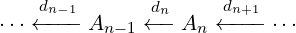
Definition 6. A chain complex (A_∙,d_∙) is a sequence of abelian groups or modules …,A₀,A₁,… connected by group homomorphisms (called boundary operators or differentials) d_n : A_n → A_n-1 such that the compositions of any two maps is the zero map (d_n ∘ d_n+1 = 0).

dn-1 dn dn+1 ⋅⋅⋅← --- An-1 ←- An ←--- ⋅⋅⋅

Example 4. A₁ = (ℤ,+) is the group of integers under addition
A₀ = (ℤ∕2ℤ,+) is the cyclic group of integers mod 2 under addition
A_n = 0 is the zero group for all n ⁄∈{0,1}. d₁(x) = x (mod 2)
d_n(x) = 0 for all n≠1

mod 2 ⋅⋅⋅0 ← 0 ← (ℤ∕2ℤ, +) ←----- (ℤ, +) ← 0 ← 0⋅⋅⋅

Since d₂ ∘ d₁(x) = d₁(0) = 0, and d_n ∘ d_n+1 = 0 by inspection for all other n, this is clearly a chain complex.

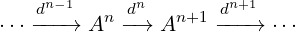
Definition 7. A cochain complex (A^∙,d^∙) is a sequence of abelian groups or modules …,A⁰,A¹,… connected by homomorphisms dⁿ : Aⁿ → Aⁿ⁺¹ such that the compositions of any two maps is the zero map (dⁿ⁺¹ ∘ dⁿ = 0).

dn- 1 n dn n+1 dn+1 ⋅⋅⋅---→ A -→ A ---→ ⋅⋅⋅

Example 5. For any p ∈ ℤ^≥2
A⁰ = (ℤ,+)
A¹ = (ℤ,+)
A² = (ℤ∕pℤ,+)
Aⁿ = 0 for all n ⁄∈{0,1,2}
d⁰(x) = p × x
d¹(x) = x (mod p)
dⁿ(x) = 0 for all n ⁄∈{0,1}

×p mod p ⋅⋅⋅0 → 0 → (ℤ, +) --→ (ℤ, +) -----→ (ℤ ∕pℤ,+ ) → 0 → 0 → ⋅⋅⋅

Remark 1. Here are some clarifying remarks about (co)chain complexes:

They are infinitely long in both directions. If you call a (co)chain complex finitely long, then you are suggesting that everything that comes before and after in the chain is the zero group.
As a consequence, they have no beginning or end unless you are not counting the infinitely long chains of zero groups that come before or after.
(Co)chain groups don’t need to have the zero group at all! They can be infinitely long and just have non-zero groups that extend in both directions.

4. Cohomology Groups

Now, we show how these groups can be computed in order to study topological spaces.

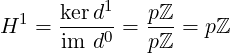
Example 6. Using the cochain complex example from above, we see that the kernel of d¹(x) = x (mod p) is just the set pℤ ⊂ ℤ. The image of d¹(x) = px is pℤ. That means the quotient group H¹ is

H1 = ker-d1= pℤ-= pℤ im d0 pℤ

Definition 10. The standard n-simplex is the convex set Δⁿ ⊂ ℝⁿ⁺¹ consisting of all (n + 1)-tuples (t₀,…,t_n) of real numbers with

ti ≥ 0 and t0 + t1 + ⋅⋅⋅+ tn = 1.

Simplices show up quite often in the study of geometric structures, and their visualizations are very friendly.

Example 8. The 1-simplex consists of the line segment connecting the points (1,0) and (0,1) including the endpoints.

Definition 11. A singular n-simplex in a topological space X is a continuous map σ from the standard n-simplex Δⁿ to X, written σ : Δⁿ → X. The i-th face of a singular n-simplex σ is the singular (n-1)-simplex

n-1 σ ∘ϕi : Δ → X

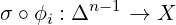
where the linear imbedding ϕ_i : Δ^n-1 → Δⁿ is defined by

ϕ (t ,...,t ,t ,...,t ) = (t,...,t ,0,t ,...,t ). i 0 i-1 i+1 n 0 i-1 i+1 n

We denote the set of all n-simplices in X as Sin_n(X). Note that Sin_n(X) = 0 for n < 0.

Definition 12. The singular chain complex of a topological space X, denoted (C_∙(X),d_∙) is created where C_n(X) is the free abelian group created by the basis Sin_n(X) and d_n : C_n(X) → C_n-1(X) is d_n(σ) = ∑ _i(-1)ⁱσ∣ [v0,⋅⋅⋅ ,ˆvi,⋅⋅⋅ ,vn] .

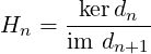
Definition 13. The nth singular homology group is the nth homology group of the nth singular chain complex.

Definition 14. The cochain group Cⁿ(X;Λ) is defined to be the dual module Hom_Λ(C_n(X;Λ),Λ) consisting of all Λ-linear maps from C_n(X;Λ) to Λ.

Definition 15. The coboundary of a cochain c ∈ Cⁿ(X;Λ) is defined to be the cochain δc ∈ Cⁿ⁺¹(X;Λ) whose value on each (n + 1)-chain a is determined by the identity

⟨δc,a⟩+ (- 1)n⟨c,da⟩ = 0.

Definition 16. The singular cohomology groups of X is defined as

Hn (X; Λ ) = Zn (X; Λ)∕Bn (X; Λ ) = (kerd)∕dCn -1(X; Λ).

We can think of Bⁿ(X;Λ) as the coboundary of the cochain group C^n-1(X;Λ) which is a subset of Cⁿ(X;Λ).

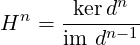
Remark 2. Cohomology groups are determined algebraically by homology groups. Here are the steps to do so:

Take a chain complex of singular, simplicial, or cellular chains.
Take the homology groups of the chain complex, kerd∕im d.
Replace the chain groups C_n by the dual groups Hom(C_n,G) and the boundary maps d by their dual maps δ.
Then, the cohomology groups are kerδ∕im δ.

5. Stiefel-Whitney Classes

Finally, we have a sufficient understanding to grasp what characteristic classes are. Primarily, we are interested in various characteristic classes because they are used to measure vector bundles of a topological space using cohomology. To do this, we map the principal bundles of a topological space X to its cohomology classes. This mapping can be done in many different ways, but in this paper we will look at the Steifel-Whitney Classes.

Definition 17. Hⁱ(B;G) denotes the i-th singular cohomology group of topological space B with coefficients in G.

Axiom 1. To each vector bundle ξ there corresponds a sequence of cohomology classes

i wi(ξ) ∈ H (B (ξ);ℤ∕2 ),i = 0,1,2,...

called the Stiefel-Whitney classes of ξ. The class w₀(ξ) is equal to the unit element

0 1 ∈ H (B (ξ);ℤ∕2)

and w_i(ξ) equals zero for i greater than n if ξ is an n-plane bundle.

Axiom 2. (Naturality) If f : B(ξ) → B(η) is covered by a bundle map from ξ to η, then

wi(ξ) = f*wi(η).

Axiom 3. (The Whitney Product Theorem) If ξ and η are vector bundles over the same base space, then

∑k wk(ξ ⊕ η) = wi(ξ)∪ wk-i(η). i=0

Axiom 4. For the line bundle γ₁¹ over the circle P¹, the Stiefel-Whitney class w₁(γ₁¹) is non-zero.

Proposition 2. If ϵ is a trivial vector bundle, then w_i(ϵ) = 0 for i > 0. This is because there exists a bundle map from ϵ to a vector bundle over a point.

Proposition 4. If ξ is an ℝⁿ-bundle with a Euclidean metric which possesses a nowhere zero cross-section, then w_n(ξ) = 0. If ξ possesses k cross-sections which are nowhere linearly dependent, then

wn -k+1(ξ) = wn -k+2(ξ) = ⋅⋅⋅ = wn(ξ) = 0.

Example 9. Using the standard imbedding of Sⁿ ⊂ ℝⁿ⁺¹, the normal bundle v is trivial. Let τ be the tangent bundle of the unit sphere Sⁿ. Then by the Whitney Product theorem, w(τ)w(v) = 1 and since v is trivial, w(v) = 1. Thus, w(τ) = 1. Therefore, the class w(τ) = w(Sⁿ) is equal to 1, and τ is indistinguishable from the trivial bundle over Sⁿ by Steifel-Whitney classes.

Theorem 3. The Whitney sum τ ⊕ϵ¹ is isomorphic to the (n + 1)-fold Whitney sum γ_n¹ ⊕γ_n¹ ⊕ ⋅⋅⋅ ⊕ γ_n¹. Hence the total Stiefel-Whitney class of Pⁿ is given by

( ) ( ) ( ) w(P n) = (1 + a)n+1 = 1 + n+ 1 a + n + 1 a2 + ⋅⋅⋅+ n+ 1 an. 1 2 n

6. Applications and Examples

Definition 18. A smooth map f : M → N between smooth manifolds is called an immersion if the Jacobian

Df : DM → DN X X f(x)

maps the tangent space DM_X injectively for each x ∈ M.

If a manifold M of dimension n can be immersed in the Euclidean space ℝ^n+k, then the Whitney duality theorem implies that the dual Stiefel-Whitney classes are zero for i > k.

6.1. Stiefel-Whitney Numbers. Stiefel-Whitney numbers allows for a comparison between the Stiefel-Whitney classes of two different manifolds. In studying manifolds, we consider the collection of all possible Stiefel-Whitney numbers. We say that two different manifolds M and M′ have the same Stiefel-Whitney numbers if

Theorem 5. If B is a smooth compact (n + 1)-dimensional manifold with boundary equal to M, then the Stiefel-Whitney numbers of M are all zero.

Theorem 6. If all the Stiefel-Whitney numbers of a manifold M are zero, then M can be realized as the boundary of some smooth compact manifold.

Corollary 1. Two smooth closed n-manifolds belong to the same cobordism class if and only if all of their corresponding Stiefel-Whitney numbers are equal.

7. Closing Remarks

To close, vector bundles themselves are quite fascinating, however it’s when we begin to construct groups with vector bundles that we see these magical algebraic properties of manifolds arise. Cohomology groups, while quite novel at first, do become a natural consideration. This is because we extract new relationships between spaces by way of the algebraic structure of cohomology classes of vector bundles. After the Stiefel-Whitney classes, there are many paths for further research after this paper. For example, one can explore vector bundles and manifolds in ℂ, which gives the added benefit of being algebraically closed. Then, one could study Chern classes and Chern numbers of a compact complex manifold.